Calorimetry again – yay or nay?
So this is the fourth time I’ve done calorimetry in class, but to be honest, I always have to refresh my knowledge on the topic every time because the concept is quite tricky at least for me. And yay at least this time there are a few changes in the methodology that we did compared to the other calorimetry experiments I’ve done before. 1.) We used a thermocouple for measuring temperatures so yay for more accurate readings, 2.) We plotted the exponential decay of temperature over time when calibrating the calorimeter instead of simple getting one temperature, which will be discussed why (woah it feels more Physics-y!)
First, we recall the following equation:![]()
Which basically governs everything that we will do here. Note that c is the specific heat capacity, which means the amount of heat required to raise per gram of a material by 1 degree Celsius. Heat capacity, C, is simply the specific heat capacity already multiplied by the mass, m, of a system. It is the heat capacity that we will determine in the calibration of the calorimeter.
In our experiment, we used a coffee cup calorimeter partially filled with water. Given that there is no escape of heat, we say that the following if correct:
![]()
Our set up looked like this:

In the calibration, we have hot water as our sample. So basically, we mixed hot water on the tap water. In a perfect situation, the final temperature when the two are mixed is supposed to be constant through time, like this:

Unfortunately, this is not always the case because the reaction is not instantaneous, and the graph looks more like this:
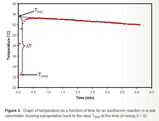
In our experiment, we accounted for the exponential decay of the temperature through time, so we plotted the logarithm of temperature vs. time to get a linear plot, then extracted the initial temperature by getting the exponential of the y-intercept. We did this for three trials and obtained an average of 926.798 J/degree Celsius for the heat capacity of the calorimeter.
Now that we have determined the heat capacity of the calorimeter, we can now use it to test two metals.
Going back to equation 2, where the sample, is now one of the metals, and using equation 1 which relates the heats to heat capacities, we are able to get the specific heat capacities of the samples. We did three trials for each to get better results and compared them to theoretical values.
